MATLAB Simulation of a 6-DOF Collaborative Robot (D-H Parameters)
MATLAB simulation of a 6-DOF collaborative robot
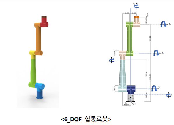
Ⅰ. D-H parameters
- D-H parameters are the parameters of a kinematic modeling method that mathematically expresses the relationship between connected links, such as those of a robot arm in mechanical engineering. There are four parameters in total, and each one describes the relationship between the coordinate frames of two links by defining a frame on each link. Before deriving the D-H parameters, the coordinate frames are set up. The origin of each joint frame is set at point Oi, and the Z-axis is placed along the axis about which each joint moves. The Z-axis is chosen along the robot’s rotation axis using the right-hand rule, with the thumb pointing along Z. With Z chosen by the right-hand rule, the index finger points along the X-axis; this X-axis lies in the plane perpendicular to both the Zi-1 and Zi axes, pointing outward from Zi-1, passing through Oi, and perpendicular to Zi. The Y-axis is then determined from the Z and X axes by the right-hand rule. To simplify the D-H parameters, the end effector, which has no rotation axis, should where possible be set in the same direction as the previous axis. Once the frames are set, deriving the D-H parameters requires understanding the relationship between each pair of frames. The D-H parameters are d, θ, a, and α, with the following meanings.
D-H parameters
-
d : the shortest distance between the Xi and Xi+1 axes, measured along the Zi axis
-
θ : the angle between the Xi and Xi+1 axes, measured about the Zi axis
-
a : the shortest distance between the Zi and Zi+1 axes, measured along the Xi axis
-
α : the angle between the Zi and Zi+1 axes, measured about the Xi axis
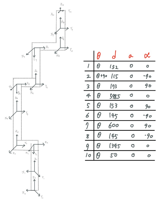
6 axis D-H parameters
\[A_{i-1}^{i} = \left[\begin{array}{} cos(\theta_i) & cos(\alpha_i)sin(\theta_1) & sin(\alpha_i)sin(\theta_i) & a_icos(\theta) \\ sin(\theta_i) & cos(\alpha_i)cos(\theta_i) & -sin(\alpha_i)cos(\theta_i) & a_isin(\theta_i) \\ 0 & sin(\alpha_i) & cos(\alpha_i) & d_i \\ 0 & 0 & 0 & 1 \end{array}\right]\]translation matrix
Ⅱ. Transformation matrix from the base frame $(x_{0},y_{0},z_{0})$ to the end effector
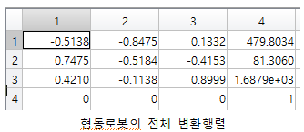
After setting up the frames and deriving the D-H parameters, they are substituted into the translation matrix to compute the T matrix. The T matrix consists of a rotation matrix and a position matrix. The rotation matrix is a 3 x 3 matrix obtained by composing the rotations in the roll, pitch, and yaw directions, and the position matrix is a 3 x 1 matrix of X, Y, Z; to match dimensions, the full matrix is 4 x 4. Substituting the D-H parameters into the T matrix expresses the relationship from joint 0 to joint 1, from joint 1 to joint 2, and so on, up to the relationship from joint n-1 to joint n. Multiplying these T matrices from T_0_1 through T_n-1_n gives the relationship (rotation and position) from the initial frame to the desired end effector.
Overall transformation matrix (orientation matrix in frame n, position vector in frame n)
Ⅲ. MATLAB simulation program that expresses the joint angle of each link using forward kinematics
- The MATLAB simulation consists of 2 function .m files and 3 executable .m files. Among the function files, theta.m expresses as a function the matrix into which the D-H parameters are substituted to compute the T matrix, and ficture.m takes the D-H parameters as direct input, uses the function in theta.m to draw the plot showing the position of each link and joint, and additionally displays the coordinates of the end effector. DOF_6.m displays the default pose of ficture.m: the D-H variables θ1 through θ6 are set to a default of 0 to show the initial pose of the collaborative robot. DOF_6_exe.m lets the user enter the variables directly. If the user input is Y or y, the same value is applied to each θn, the number of iterations is read, and the overall shape of the robot is drawn in sequence starting from the initial state, with the poses overlaid. If the user enters N or n, only a single robot shape is displayed; each θn value is read individually so that the plot can be observed as it changes with θn. Fun_Link.m expresses the robot shape as it changes with the loop value on line 5. With a unified color for links and joints, it shows the overall outline of the robot somewhat better than DOF_6_exe.m. If the axis ranges are limited in MATLAB to adjust the plot proportions, the robot shape is not drawn when it exceeds the axis range. Commenting out the axis section in each MATLAB file loses the proportions but guarantees that the end effector is always drawn. (Among the coordinates output by MATLAB, the value –7.164e-15 is effectively 0.)
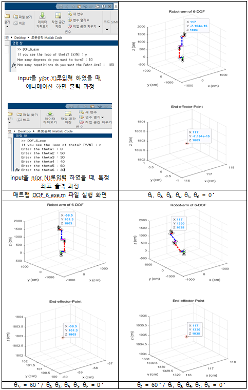
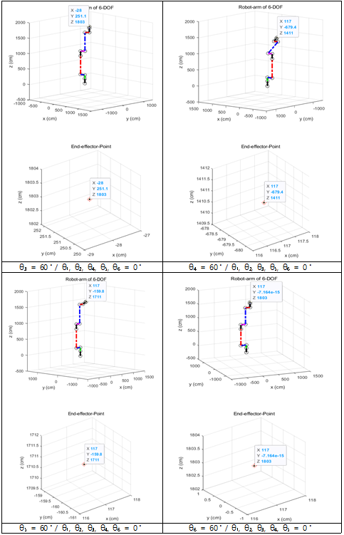
Matlab Simulation result
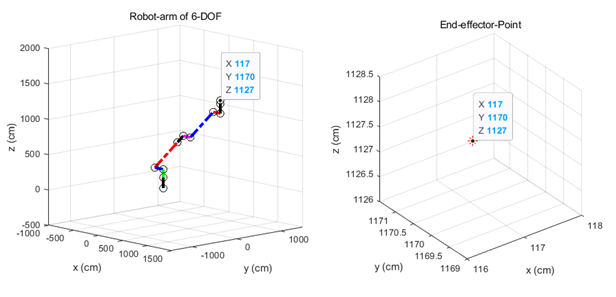
It is necessary to verify that the simulation implemented in MATLAB produces the same result as the actual calculation. Therefore θn = 60 is used as in the simulation, the transformation matrix is computed from the D-H parameter values, and the resulting position vector (X,Y,Z) is checked against the end effector position. For example, the verification is carried out with θ2 = 60, θ5 = 60.
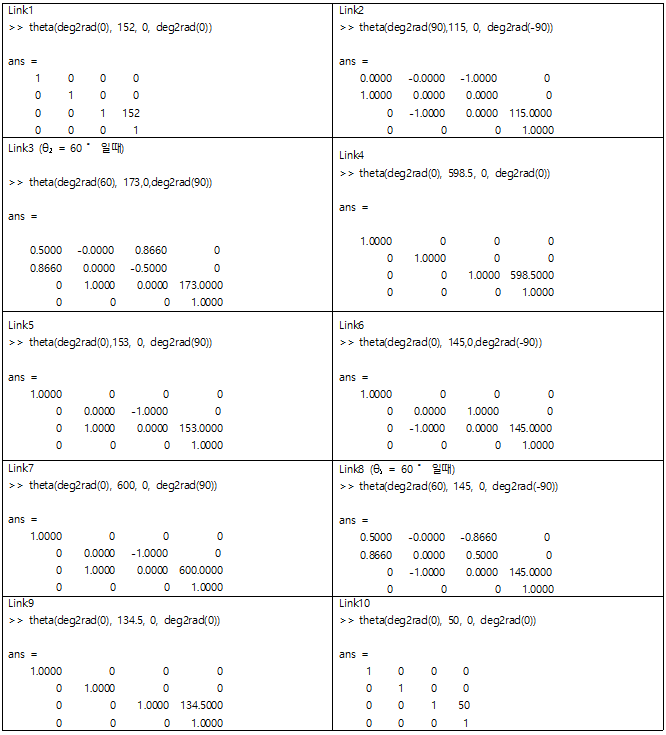
Multiplying all the link matrices gives
\[A = 10^3 \begin{bmatrix}0&-0.001&0&0.117 \\ 0.001 & 0 & 0 & 1.1704 \\ 0 & 0 & 0.001 & 1.1272 \\ 0 & 0 & 0 & 0.001 \end{bmatrix}\]Since the position vector is 117, 1170, 1127, the end effector coordinates are (X,Y,Z) = (117, 1170, 1127). This matches the simulation result.
Ⅴ. End effector path of the robot arm using cubic spline path planning
- For path planning, the current position and the goal position are set, and a path connecting the two points is planned. There are many paths connecting two points; when setting the path a robot normally follows, the aim is to reach the goal position quickly and stably. A straight line directly connecting the start and goal positions is indeed the fastest path, but the actual motion of a robot along a straight line between two points is not always stable. When running a program that tracks the actual robot path with PD control, the robot passes exactly through each waypoint and then turns to set its heading toward the next waypoint. Likewise, for a robot arm, moving directly in a straight line between points is not stable.
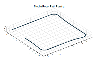
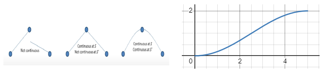
- In addition, a robot cannot operate through a stop, constant-velocity, stop sequence when moving. Therefore, to set the path through the actual stop, acceleration, constant velocity, deceleration, stop sequence and achieve smooth motion, a cubic spline is used. The cubic spline conditions are that the angle is 0 at the robot’s start position and the angular velocity is also 0. At the goal point the position has a set value, but the angular velocity is likewise set to 0. As in the left figure below, the function cannot be discontinuous at any point. To carry out acceleration and deceleration while satisfying these conditions, the change in the Y-axis (angle) with respect to the X-axis (time) can be expressed as in the right figure below.
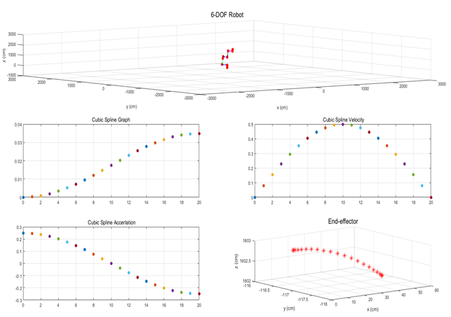
- In the actual simulation, the overall shape of the 6-DOF collaborative robot and the moving angle were driven by the input value of θ3. The position, velocity, and acceleration of the cubic spline are plotted against time, and the last graph shows the position of the end effector. The cubic spline function was set as follows.
Ⅵ. Inverse kinematics simulation code that computes the joint angles tracking the given path
- Inverse kinematics is the process of computing θ from the current end effector pose when the robot’s position is defined, by using the atan2 function on the end effector position to work backward through the tilted angles. atan2 is used because atan has θ restricted to 0 ~ 2π, so tanθ diverges at π, whereas atan2 has θ in -π ~ π and tanθ has no discontinuous interval.
Because a is 0 in the transformation matrix, the value of tanθ in the position vector is undefined, so the inverse kinematics cannot be computed.